OpenCV3-Python中meanShift和CAMShift算法应用

admin 于 2018年09月13日发表在计算机视觉

1. 均值漂移

均值漂移(Meanshif)是一种基于概率密度分布的跟踪算法，该算法一直沿着概率梯度上升的方向，迭代收敛到概率密度分布的局部峰值上，因此该算法可给出目标移动的方向。

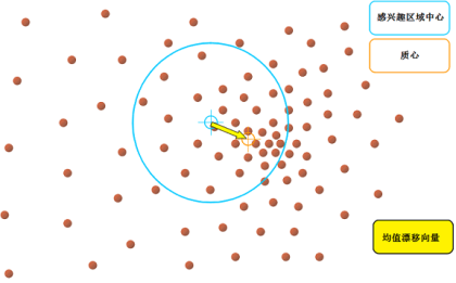
均值漂移在跟踪视频中感兴趣区域非常有用。例如：若预先不知道所要跟踪的区域，可采用这种巧妙的方法，开发程序来设定条件（颜色范围等），使应用能动态地开始（停止）跟踪视频的某些区域。

实际应用中，可采用训练好的SVM进行目标检测，同时使用均值漂移跟踪检测到的目标。

（1）程序源码

利用均值滤波窗口搜索指定颜色范围的物体，若指定颜色范围的目标进入窗口，则该窗口就会开始跟踪这个目标，否则窗口会抖动。

import numpy as np
import cv2

cap = cv2.VideoCapture(0)

# take first frame of the video
ret,frame = cap.read()

# setup initial location of window
r,h,c,w = 10,200,10,200  # simply hardcoded the values
track_window = (c,r,w,h)

#提取ROI并将其转换为HSV色彩空间
roi = frame[r:r+h,c:c+w]
hsv_roi =  cv2.cvtColor(frame, cv2.COLOR_BGR2HSV)

mask = cv2.inRange(hsv_roi, np.array((0., 0.,0.)), np.array((255.,255.,255.)))

'''
hist = cv.calcHist(images, channels, mask, histSize, ranges[, hist[, accumulate]]	)
Parameters
    images     ->  Source arrays. They all should have the same depth, CV_8U, CV_16U or CV_32F , and the same size. Each of them can have an arbitrary number of channels.
    channels   ->  List of the dims channels used to compute the histogram. The first array channels are numerated from 0 to images[0].channels()-1 , the second array channels are counted from images[0].channels() to images[0].channels() + images[1].channels()-1, and so on.
    mask       ->  Optional mask. If the matrix is not empty, it must be an 8-bit array of the same size as images[i] . The non-zero mask elements mark the array elements counted in the histogram. 
    histSize   ->  Array of histogram sizes in each dimension.
    ranges     ->  Array of the dims arrays of the histogram bin boundaries in each dimension. When the histogram is uniform ( uniform =true), then for each dimension i it is enough to specify the lower (inclusive) boundary L0 of the 0-th histogram bin and 
                  the upper (exclusive) boundary UhistSize[i]−1 for the last histogram bin histSize[i]-1 . That is, in case of a uniform histogram each of ranges[i] is an array of 2 elements. When the histogram is not uniform ( uniform=false ), then each of ranges[i] contains histSize[i]+1 elements: L0,U0=L1,U1=L2,...,UhistSize[i]−2=LhistSize[i]−1,UhistSize[i]−1 . 
                  The array elements, that are not between L0 and UhistSize[i]−1 , are not counted in the histogram.
    hist       ->  Output histogram, which is a dense or sparse dims -dimensional array.
    accumulate ->  Accumulation flag. If it is set, the histogram is not cleared in the beginning when it is allocated. This feature enables you to compute a single histogram from several sets of arrays, or to update the histogram in time.
    用于计算图像roi_hist的彩色直方图。它的x轴是色彩值，y轴是相应色彩的像素值
'''
roi_hist = cv2.calcHist([hsv_roi],[0],mask,[180],[0,180])

cv2.normalize(roi_hist,roi_hist,0,255,cv2.NORM_MINMAX)

#一种指定均值漂移终止系列计算行为的方式
term_crit = ( cv2.TERM_CRITERIA_EPS | cv2.TERM_CRITERIA_COUNT, 10, 1 )

while True:
    ret,frame = cap.read()
    
    if ret == True:
        
        #得到HSV数组
        hsv = cv2.cvtColor(frame, cv2.COLOR_BGR2HSV)
        
        '''
        dst	=	cv.calcBackProject(images, channels, hist, ranges, scale[, dst]	)
        Parameters
        images	   ->  Source arrays. They all should have the same depth, CV_8U, CV_16U or CV_32F , and the same size. Each of them can have an arbitrary number of channels.
        channels   ->  The list of channels used to compute the back projection. The number of channels must match the histogram dimensionality. The first array channels are numerated from 0 to images[0].channels()-1 , the second array channels are counted from images[0].channels() to images[0].channels() + images[1].channels()-1, and so on.
        hist	   ->  Input histogram that can be dense or sparse.
        ranges	   ->  Array of arrays of the histogram bin boundaries in each dimension. See calcHist .
        scale	   ->  Optional scale factor for the output back projection.
        直方图反向投影，其可得到直方图并将其投影到一幅图像上，其结果是概率，即每个像素属于起初那副生成直方图的图像概率。相当于等于或类似于模型图像，产生原始直方图图像的概率。
        '''
        dst = cv2.calcBackProject([hsv],[0],roi_hist,[0,180],1)
        
        #均值漂移算法
        ret, track_window = cv2.meanShift(dst, track_window, term_crit)
        x,y,w,h = track_window
        img2 = cv2.rectangle(frame,(x,y),(x+w,y+h), 255,2)
        
        cv2.imshow('img2',img2)
        if cv2.waitKey(100) & 0xff == ord("q"):
            break

    else:
        break

cv2.destroyAllWindows()
cap.release()

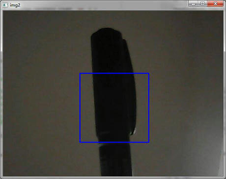
（2）实验结果

2. CAMShift算法

CamShift算法全称是“Continuously Adaptive Mean-Shift”（连续自适应MeanShift算法），是对MeanShift算法的改进算法，可随着跟踪目标的大小变化实时调整搜索窗口的大小，具有较好的跟踪效果。

（1）算法实现

Opencv中实现时，只需将上面例程中的meanShift()函数改为CAMShift()函数即可。

原始内容：

 #均值漂移算法
 ret, track_window = cv2.meanShift(dst, track_window, term_crit)
 x,y,w,h = track_window
 img2 = cv2.rectangle(frame,(x,y),(x+w,y+h), 255,2)

更改后内容：

 #CAMShift算法
 ret, track_window = cv2.CamShift(dst, track_window, term_crit)
 pts = cv2.boxPoints(ret)
 pts = np.int0(pts)
 img2 = cv2.polylines(frame,[pts],True, 255,2)

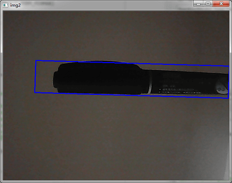
（2）实验结果